Railroad Stock – Discovering Opportunities

The fundamental rule of investing is to buy low and sell high. Unfortunately, an investor doesn’t know when either a low or a high price is going to happen. What if the price drops for the stock and you buy it, and then it keeps dropping? When do you sell? Nobody has a crystal ball that can foretell the future. You have to base your decisions on facts and the most likely outcomes based on the historical behavior of the investment.

One of the benefits of railroad stocks is the downside risk. When the stock’s share price decreases, it is unlikely will continue falling. The business ratios used in this industry assist in understanding how far a share price can fall. The further the price decreases, the more lucrative the investment becomes. Thus, the market, other buyers are enticed to purchase the stock due to the desirable attributes of the stock. The first section below covers this particular aspect of the share price decrease.

On the flip side are increases in share price. How does an investor know when to sell? If you sell early, you miss out on any additional increases in share price that can add dramatically to your gain upon the sale of the stock. With railroad stock, the historical pattern has rarely wavered from a continuously increasing trend line. The key is to be patient. Yes, the longer it takes to recover and generate gains for the investor, the lower the yield for the investor. Never look at this in isolation; it’s about Bernoulli’s Law (Law of Large Numbers). In the long run, if you adhere to the model, you will make positive gains, I’m talking about 18 to 30% year on year, not sudden 40 to 50% gains. The second section explores triggers to sell the stock; how do you know when it’s time?

This is where railroad stocks are ideal for the application of this concept. As stated in the prior article in this series, railroad stocks are solid and steady investments. There are six companies publicly traded with sufficient revenue and similar operational systems for comparative purposes. In addition, each company provides a plethora of information to assist the investor in understanding the downside risk and, of course, the pattern and underlying circumstances that push upward on the share price. The final section illustrates the development of a model. In this case, I use Kansas City Southern’s history and walk the investor through the steps necessary to develop the decision model.

Railroad Stocks – Limited Downside Risk

One ratio stands out in determining downside risk for a stock. It is the price-to-book ratio. The price-to-book ratio compares the market price of a share of stock against the book value of that same stock. The most important value of this ratio is the actual book value. It is important to understand that book values can be solid, assuming the only asset is cash, or risky, assuming the only assets are junk bonds.

With railroad companies, book value is focused on the primary assets, which are fixed in nature (read the 2nd article in this series). Fixed assets comprise at least 85% of all assets. The fixed assets are subdivided into several types:

Land
Track/Roadway Access
Rail Cars/Locomotives
Buildings
Technology

Typically, land is 5% of the fixed assets. Land was recorded at cost many years ago; thus, the actual market value of the land has increased. The other fixed assets have been depreciated at reasonable rates. An investor must understand an important business attribute of these assets: they are only valuable to another railroad company. There isn’t much of a market for railroad track, rail cars, etc., to the general market other than to another railroad company.

Thus, the question is: Is the book value of a railroad stock reasonable? Reliable?

The answer is yes, why? Because of the going-concern aspect of railroad companies. Everyone has heard the proverbial statement: ‘it’s hard to stop a train’. Well, this applies to these six Class I railroads. It is nearly impossible to stop them; their operations serve unique markets, and the alternatives for their customers are way more expensive than utilizing the railroad to meet their transportation needs. Thus, the likelihood of any railroad company suddenly going out of business is remote. Even if the economy tanked, they will continue to operate, as other ratios indicate they have enough financial flexibility to absorb whopping decreases in sales.

Getting back to the price-to-book ratio, for railroad companies, this relationship simply tells the investor the potential downside risk. The lower the ratio, the less likely the share price will decrease dramatically. Here are the top six current price-to-book ratios after posting of third quarter results for 2019 (ending September 30th, 2019).

October 22, 2019
. Market Price Book Value Price to Book
Union Pacific $170.46 $25.13 6.78
CSX $71.80 $15.18 4.73
Canadian National $88.99 $25.66 3.46
Norfolk Southern $187.54 $57.65 3.25
Canadian Pacific $219.37 $52.02 4.21
Kansas City Southern $145.11 $49.89 2.91

Kansas City Southern has the lowest price-to-book ratio at 2.91. With a current book value of $49.89 per share, the company’s downside risk is relatively small. This means that as the price per share drops, it will not drop as a percentage of the recent high as higher-priced-to-book stocks. Why? The low price-to-book value makes the stock attractive to buyers. To validate this statement, let’s compare a high price to book value stock price chart against Kansas City Southern and evaluate market price decreases as a percentage of the associated high, and see if this measurement holds. For purposes of this comparison, I’m going to use CSX.

Below is CSX’s stock price chart over the last three years. Four large decreases in value are circled, and the resulting outcomes are as follows:

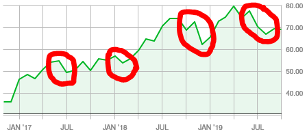
. Date High Date Low Value Change
05/13/19 $78.40 08/19/19 $64.62 – 17.57 %
11/26/18 $72.63 12/17/18 $60.70 – 16.42 %
01/08/18 $59.25 02/05/18 $50.89 – 14.11 %
07/10/17 $55.08 07/31/17 $48.74 – 11.51 %

Now, look at the results for Kansas City Southern. There are three decreases circled. The second one has two steps, which makes the total number of decreases four. The resulting outcomes are as follows:

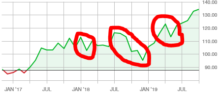
. Date High Date Low Value Change
04/29/19 $125.25 05/27/19 $113.28 – 9.56 %
09/04/18 $118.07 10/08/18 $102.57 – 13.13 %
11/26/18 $103.05 12/17/18 $92.74 – 10.01%
01/22/18 $113.50 02/05/17 $103.77 – 8.57 %

Notice the difference in the decrease in price as a percentage of the share price at the high just prior to the decrease. CSX has a greater percentage change because of the higher price-to-book ratio, i.e., there is more room for a decrease in value than Kansas City Southern. CSX’s price to book ratio of 4.67 (this was not the price to book on those dates, but CSX’s price to book was relatively much higher than Kansas City Southern’s on those respective dates) is almost double Kansas City Southern’s 2.91 (which was much lower during this time frame). Thus, a lower price-to-book ratio creates greater resistance to negative market price decreases than higher ratios.

Why is this so important? Well, when developing a buy/sell model, the investor must take into consideration the negative changes related to the respective investment. It is obvious that Kansas City Southern will have negative changes that are nowhere near as severe as the negative changes for CSX. This model assists the buyer with the buy low’ part of the formula. It assists with determining the timing of the buy.

There is another factor that comes into play: yield.

Yield refers to the dividends received as a percentage of the share price on an annual basis. It is just as simple as ‘what is the interest rate the bank pays on your savings deposit’. When you purchase the share, you are economically depositing money into a savings account. The bank, in this case the railroad company, pays dividends to the shareholders; no differently than a bank pays its customers interest on their deposits. The amount paid as a percentage of the amount invested is referred to as the yield.

As the share price increases in the market and the dividend payments stay the same, the yield decreases. As the share price drops, the yield increases and can increase at an accelerated rate as the share price continues to drop. Let’s take a look at what would happen to the yield if Norfolk Southern’s share price drops through steps over a 30% range.

Market Price on October 18, 2019, for Norfolk Southern: $181.91
Current Annual Dividend Amount: $3.45 (Estimated)
Yield: 1.897%

. Market Price Yield (Assumes no Decrease in Dividend Payment)
. $175 1.971%
. $168 2.054%
. $160 2.156%
. $150 2.300%
. $142 2.429%
. $134 2.575%
. $127 2.716%

As you can see, the yield steadily improves and becomes very attractive for longer-range investors, ones that hold the stock for many months and are willing to wait more than six months for the stock to recover and then sell or even continue to hold strictly for the yield. This is a secondary reason that the downside risk for railroad stocks is limited. The yield is attractive to buyers, and if the share price decreases, the yield begins to attract many new buyers in the market, thus dampening the downward pressure.

The final reason the downside risk is limited is the historical positive earnings pattern for all six Class I Railways. All of them earn profits even during recessions. Look at these earnings per share for five of the six companies over a ten year period; always positive, not one single negative outcome from any of them.

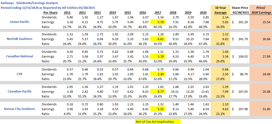
If you recall our economic history, in late 2007, early 2008, and through most of 2012, the US economy was in a state of recession. Yet these railroad companies continued to earn profits per share. NOT A SINGLE COMPANY REPORTED NEGATIVE EARNINGS DURING THIS LONG RECESSION. Go back to the second article in this series, and it will explain the financial break-even point for railroad companies and how easy it is for them to achieve financial profits.

By the way, many of you are looking at the graph and are wondering why on earth there is a sudden increase in earnings for all railroad companies in the fourth quarter of 2017? Remember that in December of 2017, the United States modified the tax rate for all corporate entities. All the companies took advantage of this reduced rate and reported more income (tax deferred items) to pay a lower tax amount. Thus, the continued step-up of earnings per share into 2019.

These three attributes of this industry minimize downward changes in share price. What is really interesting is that it is difficult to find actual significant decreases in the share price for a railroad company. When it does happen, it is time to buy the stock.

Once bought, when do you sell?

Keys to Trigger the Sale of Railroad Stock

If you apply a well-developed model, this is easy to determine.

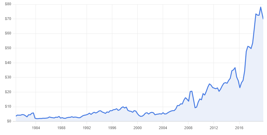
Five of the six companies follow a similar pattern with their respective stock price. Look at this graph for Union Pacific (the largest of all the railroad companies):

This is over 50 years. Union Pacific is considered a leader in the railroad industry. The company generates more than $22 billion a year in revenue, outpacing its nearest competitor by $7 billion. The share price has quadrupled over the last 10 years. The key to this chart is that any downward change recovers within a reasonable period of time. Let’s take a look at CSX and compare.

Look familiar?

Five of the six follow a very similar pattern, as illustrated with Union Pacific and CSX. However, one stands out with an odd share price line over 50 years. Here is Kansas City Southern’s share price history.

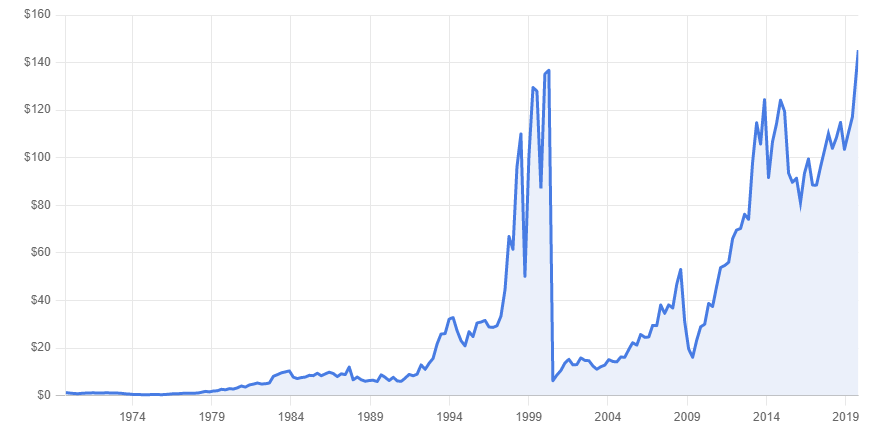
On April 11, 2000, the share price peaked at $136.75. Over three months, the price dropped to $6.25 per share. What happened?

A novice investor would think that the company did something wrong or that there was some lawsuit. Sometimes there are legitimate business reasons why this happens. In this case, Kansas City Southern spun off their financial arm. Basically, the company consisted of two divisions, a financial division and the railroad company. The company received permission from the IRS and split the company into two separate companies. The financial division generated almost 95% of the revenue. Thus, when the split occurred, the shareholders received stock in the new finance services company worth about 95% of the total share price value on the day of the split. The existing shareholders continued to own KSU, but the market value decreased to reflect the value of KSU as a railroad on that day. Review the revenues section of the comprehensive income statement for the 2nd quarter of 2000. I highlight the dollar amount associated with the financial services division.

The key is that the pattern continues for Kansas City Southern after the spin-off of the financial services division.

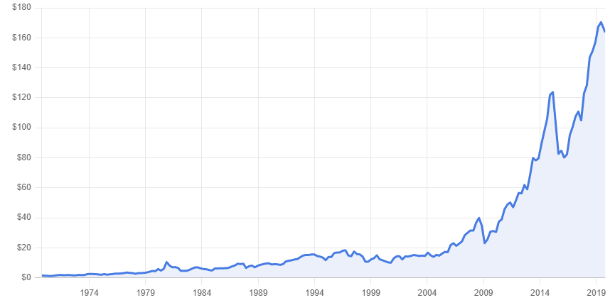
When looking at these charts, an investor would say that it appears that railroad stocks will continue on the same pattern infinitely. However, this is not the case. The railroad companies are merely mimicking the stock market. Look at the stock market value line since 1990.

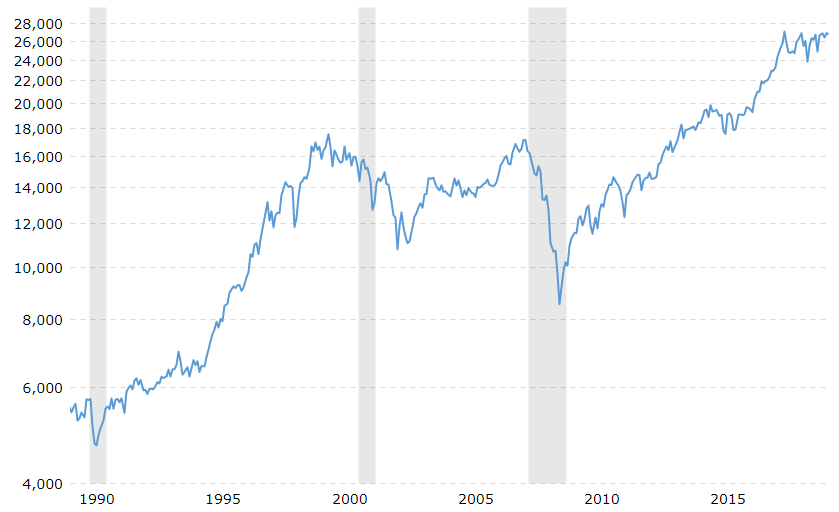
The entire market has quadrupled in the last 30 years. Thus, much of the railroad stock change is tied to the market as a whole. Again, a key indicator of stability and reliability. So how does an investor discover opportunities?

The answer is simple: when the stock price decreases by a given percentage, it is an indicator to buy. It will recover; in some situations, it may take longer than the investor desires, but it will recover to the prior value. And when it does, it’s time to take the gain and reallocate to other railroad stocks. That is, buy whenever any of the six stocks has a negative price change, and sell when it recovers.

Initial Model – Kansas City Southern

There’s an interesting law related to outcomes. The more data sampling points, the more likely the probability of predicting the outcome accurately increases. As an example, many of you read polls; the higher the number of samples, the more likely the poll is accurate. In general, a reasonable poll will need about 800 samples or responses to state an outcome within plus or minus 5%. If you increase the responses to more than 1,000, your accuracy improves to better than 3%. This is known as Bernoulli’s Law.

An investor can apply Bernoulli’s Law to buying and selling. There are plenty of data points to develop a pattern of likely outcomes. It is now a matter of application.

Thus, I’ll start out with Kansas City Southern and record all points that meet certain criteria and apply them over the last year, and measure the outcomes.

First step, build a set of criteria to force the buy/sell trigger points. Next, let’s review the outcomes.

Buy Criteria

The first important point is to determine the frequency at which to buy and sell. In general, a value investor does not want to get involved in ‘day trading’. This goes against the principle of value investing for several reasons:

Value investing is about patience and understanding that any purchase of stock at a certain price will be rewarded because the market price will generally increase given time, i.e., the underlying business dynamics and industry ratios support the outcome of market price improvement over time.
Day trading requires constant attention to the respective investments, whereas value trading is simply a matter of buying at a certain trigger point and selling at a certain trigger point. Just set the points and allow time to do the work for you.
Time is a value investor’s greatest asset.

On the other hand, value investors do not want to buy stock to simply ‘Hold’ the stock. Value investors seek out patterns that are highly reliable and produce value. The question remains, how frequently can we expect to have significant changes in a stock’s market price? To answer this, let’s first look at the past year for Kansas City Southerns’ share price in the market. Here is the graph.

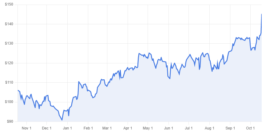
The first thought to note is the entire price range over one year. The lowest point was $90.84, and the highest was actually on the 18th of October 2019 at $145.81. A whopping $54.97 differential.

If you look at the graph, there are multiple drops and peaks throughout this period. Again, the question is, what is a reasonable frequency of change?

Let’s explore this question. If an investor quantifies change as any movement in the same direction that is greater than 10%, how many changes occur? Let’s chart this with KSU.

Again, the price must change by 10% in the same direction. Go back to October 18, 2018. The price was $106.12. Notice it slides downward until October 23, 2018, where it stops at $101.85. A 10% decrease in price from $106.12 equals $10.61. Thus, the decrease to the 23rd doesn’t meet the criterion. Notice it recovers slightly to $103.70 on the 24th. Here, the downward slide continues, where the price falls to $98.86 on the 28th of October. This does not meet the 10% test from the start when the price was $106.12. Thus, to meet the 10% test, that downward slide must have a longer line downward. If you look at the graph overall, there appear to be about 4 potential points along this line. They are circled in the following graph (same graph, just now has circles around the potential downward slides).

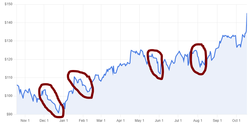
Now let’s chart these four decreases:

Date Peak Price Date Bottom Price Change in $ % Change
12/02/18 $103.55 12/23/18 $90.84 $12.71 12.27%
01/17/19 $110.52 02/07/19 $102.22 $8.30 7.51%
05/20/19 $120.62 06/02/19 $112.05 $8.57 7.10%
07/28/19 $125.00 08/04/19 $115.79 $9.21 7.37%

Of these four distinct decreases, only one qualifies with more than a 10% change. This tells us that the criterion of more than 10% is set too high. Only once a year limits the investor’s ability to keep their money working throughout the entire year. If you look at the graph, it takes about 30 plus days to recover, and if we set our minimum requirement at 10%, an investor’s money is only working 30 days per year.

Realistically, an investor wants the money to work at least half of the year. Thus, we need to reduce the downward percentage to something that will trigger buys about six times a year. If we reduce this trigger, these four points will be included in the model as they will meet the minimum requirements.

Even at 7%, this happens only four times a year that this happens. An investor wants more frequency with the model, but not too much more, as there will be too many downward points. Look at the graph; there are about 40 downward changes over a year. Let’s use 5% as the change. Let’s chart this data:

. Minimum 5% Downward Change From Prior Peak
Date Peak Price Date Bottom Price Change in $ % Change
10/18/18 $106.12 10/28/18 $98.86 7.26 6.84
11/06/18 $104.06 11/13/18 $97.20 6.86 6.59
12/02/18 $103.55 12/23/18 $90.84 12.71 12.27
01/27/19 $109.33 02/07/19 $102.22 7.11 6.50
05/05/19 $124.36 05/12/19 $117.36 7.00 5.63
05/27/19 $120.61 06/02/19 $112.05 8.56 7.09
07/28/19 $125.00 08/04/19 $115.79 9.21 7.37

Altogether, there are now seven incidences of a value change greater than 5% throughout this prior year. Therefore, we have enough frequency to justify 50% utility of the investment. However, we have to modify the results. Remember, nobody knows when it will bottom out. Our model simply states that the investor will buy when the change is greater than 5% from the previous peak, including any peaks within a few days of the prior peak, which our results above derive.

Thus, our buy points are as follows, in addition, I’m including purchase costs of 1.8%:

. Buy at 5% Downward Change From Prior Peak.
Date Peak Price Date Purchase Price Purchase Costs Total Per Share Cost
10/18/18 $106.12 10/23/18 $101.81 1.84 $103.65
11/06/18 $104.06 11/12/18 $98.86 1.78 $100.64
12/02/18 $103.55 12/06/18 $98.37 1.77 $100.14
01/27/19 $109.33 02/05/19 $103.86 1.87 $105.73
05/05/19 $124.36 05/10/19 $118.14 2.13 $120.27
05/27/19 $120.61 05/30/19 $114.59 2.06 $116.65
07/28/19 $125.00 08/03/19 $118.75 2.14 $120.89

Now that we have our buy points and frequency, let’s set the sell criteria and points tied to these respective purchases.

Railroad Stock Sell – Time to Earn Some Money

As stated earlier, if you monitor the business ratios and the companies closely, you should feel comfortable that the stock will recover. But the question now is, when do you sell? Go back to the KSU graph. Notice that 100% recovery plus more occurs about a month later. Thus, let’s start by setting our recovery requirements to a 7% increase in share price over the purchase price. Let’s look at the respective selling points financially.

. Sell at 7% Increase over Purchase Price
. Total Sell Point Net
. Date Purchase Price Purchase Costs Per Share Cost Sell Date 107% of Buy Sell Costs @1.8% Sale Proceeds Net $ Gain
10/23/18 $101.81 1.84 $103.65 01/16/19 $108.94 $1.95 $106.99 $3.34
11/12/18 $98.86 1.78 $100.64 01/16/19 $105.78 $1.91 $103.87 $3.23
12/06/18 $98.37 1.77 $100.14 01/16/19 $105.26 $1.90 $103.36 $3.22
02/05/19 $103.86 1.87 $105.73 02/20/19 $111.13 $2.00 $109.13 $3.40
05/10/19 $118.14 2.13 $120.27 09/03/19 $126.41 $2.28 $124.13 $3.86
05/30/19 $114.59 2.06 $116.65 09/03/19 $122.61 $2.21 $120.40 $3.75
08/03/19 $118.75 2.14 $120.89 09/03/19 $127.06 $2.29 $124.77 $3.88

Something interesting happens here. Notice we have overlaps. This is because another minimum 5% drop occurs while we are waiting for the stock to recover. Go look at the graph; you can see the stock price experiences several declines before it finally recovers based on the criteria set. This means that out of the seven potential purchases, we can only do three because the share price did not recover before another drop. Thus, if we agree to tie up $2,000 as our investment fund for this particular stock, let’s find out the results over one year.

. Investment of $2,000
. Total Sell Point Net
. Date Purchase Price Purchase Costs Per Share Cost Sell Date 107% of Buy Sell Costs @1.8% Sale Proceeds Net $ Gain
10/23/18 $101.81 1.84 $103.65 01/16/19 $108.94 $1.95 $106.99 $3.34
02/05/19 $103.86 1.87 $105.73 02/20/19 $111.13 $2.00 $109.13 $3.40
05/10/19 $118.14 2.13 $120.27 09/03/19 $126.41 $2.28 $124.13 $3.86

The investment begins on 10/23/18

With $2,000, the fund buys 19.295 shares and sells them for a net amount of $106.99/each on January 16, 2019, for a new fund balance of $2,064.45. These proceeds are used on 02/05/19 to buy 19.526 shares at a total cost of $105.73 each (includes trading costs). On 02/20/19, we sold these shares at $109.13 each (including costs of sales), netting $2,130.84. Almost three months later, we buy 17.717 shares at $120.27, including trading costs. Finally, at the end of the year, technically about 1.5 months before the close of this cycle, we sell these shares for $124.13 each, net of trading costs, to collect $2,199.22.

Altogether, over one year, we netted $199.22 after costs for a yield of 9.961%. However, the money was only tied up for 219 days. This means that our fund earns .0455% per day for the money that is utilized. Thus, if we were able to use the money for all 364 days, our return on the investment would have been 16.56%.

How can we make this better?

Leverage – Bernoulli’s Law

There are several tools to leverage this outcome higher with little additional risk. First, you must have a similar model for every railroad stock. Why? Think of the pooling concept, let’s assume that out of the six railroad companies, the pool has money invested in three of them. This means that in the aggregate, there will be very little unused utility related to the dollars in the pool. Let’s assume the pool is $10,000 and the maximum investment in any single purchase (notice I didn’t say company) is $2,000. This way, almost all the money will be tied up throughout the cycle. Thus, instead of a 9.961% return, the pool will leverage its investment towards a 364-day full utility. It will probably exceed 330 days per year for a total average return of 15.015%.

Secondly, and the one that stands out like an elephant in the room, are the trading costs. I used 1.8% as the cost to trade. Naturally, there is an economy of scale involved for really large purchases, i.e., retirement funds have lower costs per trade as a percentage of the investment. In general, their costs are less than .5%; a whopping 1/3 of this example’s costs. Since we are only buying about 15 to 20 shares per transaction, the key is to get that cost to less than $1 per share. At $1.00 per share, the fund pool at the end of the above cycle would be around $2,361.02. This annual return is 18.051% for a daily average of .0824 (almost double the example’s average). If this is extrapolated over 330 days of utility for each dollar in the pool, the annual return on the investment is 27.20%!

A third tool is to up the recovery requirement to a higher percentage. Let’s see what happens if we go to a 10% recovery requirement. Before I present the results, remember what happens here: we increase the risk of downward slides during the hold period because it takes more time to recover, thus bringing into play additional downward slides that require the money to be held longer in the investment. Here are the results:

. Investment of $2,000
. Total Per Sell Point Net
. Date Purchase Price Purchase Costs Share Cost Sell Date 110% of Buy Sell Costs @1.8% Sale Proceeds Net $ Gain
10/23/18 $101.81 1.84 $103.65 03/06/19 $111.99 $2.02 $109.97 $6.32
02/05/19 $103.86 1.87 $105.73 02/20/19 $111.13 $2.00 $109.13 $3.40
05/10/19 $118.14 2.13 $120.27 09/03/19 $129.95 $2.34 $127.61 $7.34

Notice something very important here: by increasing the recovery threshold to sell, the model eliminates the ability to buy at another point. In this case, the increased threshold to sell eliminates the ability to buy on 02/05/19. But still, let’s review the financial results.

With $2,000 invested on 10/23/18, the fund purchases 19.2957 shares. On March 6, 2019, the fund sells those shares for $2,121.95. With those proceeds, the fund buys 17.6432 shares and proceeds to sell them on September 3rd for $2,251.45. This holding longer concept netted an additional $52.23, making the return on the investment a flat annual 12.573%. The money was tied up for 135 days, which is .09313% per day. Notice how significantly greater this is over the .0455% with the original example. If we can tie the money up for 330 days per year (utilizing the entire six companies in a portfolio), the return on the investment would equal 30.734%.

Many of you are now thinking, Hey, hold the investment even longer, i.e., up the recovery amount. My gut is that it will not hold; there is an optimum point of maximizing return. You take away other opportunities when you do this. But let’s see what happens if we go to 12%.

. Investment of $2,000
. Total Per Sell Point Net
. Date Purchase Price Purchase Costs Share Cost Sell Date 112% of Buy Sell Costs @1.8% Sale Proceeds Net $ Gain
10/23/18 $101.81 1.84 $103.65 03/13/19 $114.03 $2.52 $111.51 $7.86
05/10/19 $118.14 2.13 $120.27 09/09/19 $132.32 $2.38 $129.94 $9.67

Wow, it did work out! We didn’t eliminate an opportunity to buy using the same funds. I’m even impressed. Let’s calculate the financial results. On 03/13/19, the fund earns $2,151.66 on the 19.2957 shares it bought on 10/23/18. On 05/10/19, the fund buys 17.89 shares. On 09/09/19, the fund receives $2,324.66 for those shares. The fund earns 16.233%. Funds were tied up for 142 days, netting a .1143% per day. If the fund can get this over 330 days, the actual return on the investment equals 37.72%.

What a surprise!

By the way, the model continues to work with increasing results to 14%. At 14% recovery, we eliminate the ability to take advantage of the decrease on 05/10/19, and thus the aggregate return drops dramatically. Therefore, it looks like a 12 to 13% recovery for KSU is the optimum recovery point. Again, this changes each year and with the quarterly reported results. I reiterate the importance of adjusting your model each quarter for each company. Each company is going to be different depending on the frequency of change. As stated in the prior section, you must have adequate frequency to maximize the use of funds, and the level of recovery can’t be too high or the utility rate of money is too low, forcing the aggregated return lower.

The next set of articles will build the models for each of the respective railroads. For now, I’m going to work with this model for KSU.

On Friday, the 18th of October, KSU’s stock price jumped higher due to the 3rd quarter results reported in their 10-Q report. For now, I’m going to go with a 5% decrease and a 12% recovery and see the results over the next year. My maximum investment (using fake dollars by the way) is $2,500. Each share will cost me $1 to trade, no matter whether I’m buying or selling. Let’s see what happens with the model. I’m expecting about a 10% return on my fund tied to this respective company. Since I’ll be pooling my money in the fund, I’ll have about 4 separate investments ongoing over the six companies for an initial investment in my pool of $10,000.

As of this report, I do not have an investment in KSU. I need to simply wait for the price to peak and see a drop of at least 5%, then I’ll start the fund investing in KSU. Act on Knowledge.